Simulating and AFM Cantilever response in Python

The simulation code integrates the ordinary differential equation describing an AFM cantilever’s motion. That, by itself, is not particularly interesting as it’s just an exercise for undergraduates in physics courses. What IS interesting, is adding some sort of transient excitation and seeing the response.

The simulation code in FFTA package allows for an excitation voltage to be applied at some particular point in time and therefore affects the cantilever’s motion. More specifically, this simulation applies a shift in the resonance frequenecy with some time constant and an electrostatic force that changes with the same time constant. By default, that time-dependent response is an exponential decay: \((1-e^{-t/\tau})\)

but that can be any callable function.

A secondary option is to apply an electric drive to the cantilever to see second resonance responses, but that is outside the scope of this notebook.

Much of this is used in the following publication: Karatay DU, Harrison JA, et al. Fast time-resolved electrostatic force microscopy: Achieving sub-cycle time resolution. Rev Sci Inst. 87, 053702 (2016). DOI: 10.1063/1.4948396

!pip install FFTA==0.3.1

Collecting FFTA==0.3.1
  Downloading https://files.pythonhosted.org/packages/aa/b8/59a1c27a19d5f8efc16ff28ae4630416581279184735b9e888203e6215e2/FFTA-0.3.1.tar.gz (89kB)
     |████████████████████████████████| 92kB 4.0MB/s
Requirement already satisfied: numpy>=1.18.1 in /usr/local/lib/python3.6/dist-packages (from FFTA==0.3.1) (1.18.5)
Requirement already satisfied: scipy>=1.4.1 in /usr/local/lib/python3.6/dist-packages (from FFTA==0.3.1) (1.4.1)
Collecting igor>=0.3
  Downloading https://files.pythonhosted.org/packages/be/f2/ad4b0027e58c78958b40d9da54e5674a9e851207a9b61e5edd4112f154ec/igor-0.3.tar.gz (51kB)
     |████████████████████████████████| 61kB 8.6MB/s
Requirement already satisfied: numexpr>=2.7.1 in /usr/local/lib/python3.6/dist-packages (from FFTA==0.3.1) (2.7.1)
Collecting watchdog>=0.10.2
  Downloading https://files.pythonhosted.org/packages/6f/10/500580a0987363a0d9e1f3dd5cb1bba94a47e19266c6ce9dfb6cdd455758/watchdog-0.10.4.tar.gz (98kB)
     |████████████████████████████████| 102kB 9.9MB/s
Collecting pyUSID>=0.0.8
  Downloading https://files.pythonhosted.org/packages/3f/5e/cb92d9532f404fd271236254a31902725cc957d1ac3aea3ebe10b938f8f3/pyUSID-0.0.9-py2.py3-none-any.whl (166kB)
     |████████████████████████████████| 174kB 41.0MB/s
Collecting pycroscopy>=0.60
  Downloading https://files.pythonhosted.org/packages/7a/cd/52861a55bff7f7f8582a1c4df1df8f4dfa3bb828011f55da82d201215030/pycroscopy-0.60.7-py2.py3-none-any.whl (354kB)
     |████████████████████████████████| 358kB 48.5MB/s
Requirement already satisfied: pywavelets>=1.1.1 in /usr/local/lib/python3.6/dist-packages (from FFTA==0.3.1) (1.1.1)
Collecting sidpy>=0.0.2
  Downloading https://files.pythonhosted.org/packages/13/83/8c08b60f3003428345a1234db9e2362cfbde75175bddabbf18b692fb60d5/sidpy-0.0.3-py2.py3-none-any.whl (74kB)
     |████████████████████████████████| 81kB 10.6MB/s
Collecting pathtools>=0.1.1
  Downloading https://files.pythonhosted.org/packages/e7/7f/470d6fcdf23f9f3518f6b0b76be9df16dcc8630ad409947f8be2eb0ed13a/pathtools-0.1.2.tar.gz
Requirement already satisfied: pillow in /usr/local/lib/python3.6/dist-packages (from pyUSID>=0.0.8->FFTA==0.3.1) (7.0.0)
Requirement already satisfied: dask>=0.10 in /usr/local/lib/python3.6/dist-packages (from pyUSID>=0.0.8->FFTA==0.3.1) (2.12.0)
Requirement already satisfied: toolz in /usr/local/lib/python3.6/dist-packages (from pyUSID>=0.0.8->FFTA==0.3.1) (0.11.1)
Requirement already satisfied: matplotlib>=2.0.0 in /usr/local/lib/python3.6/dist-packages (from pyUSID>=0.0.8->FFTA==0.3.1) (3.2.2)
Requirement already satisfied: six in /usr/local/lib/python3.6/dist-packages (from pyUSID>=0.0.8->FFTA==0.3.1) (1.15.0)
Requirement already satisfied: ipywidgets>=5.2.2 in /usr/local/lib/python3.6/dist-packages (from pyUSID>=0.0.8->FFTA==0.3.1) (7.5.1)
Collecting ipython>=6.0; python_version >= "3.3"
  Downloading https://files.pythonhosted.org/packages/23/6a/210816c943c9aeeb29e4e18a298f14bf0e118fe222a23e13bfcc2d41b0a4/ipython-7.16.1-py3-none-any.whl (785kB)
     |████████████████████████████████| 788kB 45.4MB/s
Requirement already satisfied: psutil in /usr/local/lib/python3.6/dist-packages (from pyUSID>=0.0.8->FFTA==0.3.1) (5.4.8)
Collecting cytoolz
  Downloading https://files.pythonhosted.org/packages/58/67/1c60da8ba831bfefedb64c78b9f6820bdf58972797c95644ee3191daf27a/cytoolz-0.11.0.tar.gz (477kB)
     |████████████████████████████████| 481kB 45.6MB/s
Requirement already satisfied: joblib>=0.11.0 in /usr/local/lib/python3.6/dist-packages (from pyUSID>=0.0.8->FFTA==0.3.1) (0.17.0)
Requirement already satisfied: h5py>=2.6.0 in /usr/local/lib/python3.6/dist-packages (from pyUSID>=0.0.8->FFTA==0.3.1) (2.10.0)
Collecting numpy-groupies==0.9.7
  Downloading https://files.pythonhosted.org/packages/4c/18/e5c4c6d12ef8740106d29ea78bad2c1d218e61caa735513d3491a3a1d837/numpy_groupies-0.9.7.tar.gz
Requirement already satisfied: scikit-image>=0.12.3 in /usr/local/lib/python3.6/dist-packages (from pycroscopy>=0.60->FFTA==0.3.1) (0.16.2)
Requirement already satisfied: scikit-learn>=0.17.1 in /usr/local/lib/python3.6/dist-packages (from pycroscopy>=0.60->FFTA==0.3.1) (0.22.2.post1)
Requirement already satisfied: xlrd>=1.0.0 in /usr/local/lib/python3.6/dist-packages (from pycroscopy>=0.60->FFTA==0.3.1) (1.1.0)
Collecting gwyfile
  Downloading https://files.pythonhosted.org/packages/28/a8/7e1f5105cbf8200705f130545c9ad54592c52c34717609f87570e5a5e2af/gwyfile-0.2.0-py2.py3-none-any.whl
Requirement already satisfied: pyparsing!=2.0.4,!=2.1.2,!=2.1.6,>=2.0.1 in /usr/local/lib/python3.6/dist-packages (from matplotlib>=2.0.0->pyUSID>=0.0.8->FFTA==0.3.1) (2.4.7)
Requirement already satisfied: cycler>=0.10 in /usr/local/lib/python3.6/dist-packages (from matplotlib>=2.0.0->pyUSID>=0.0.8->FFTA==0.3.1) (0.10.0)
Requirement already satisfied: python-dateutil>=2.1 in /usr/local/lib/python3.6/dist-packages (from matplotlib>=2.0.0->pyUSID>=0.0.8->FFTA==0.3.1) (2.8.1)
Requirement already satisfied: kiwisolver>=1.0.1 in /usr/local/lib/python3.6/dist-packages (from matplotlib>=2.0.0->pyUSID>=0.0.8->FFTA==0.3.1) (1.3.1)
Requirement already satisfied: widgetsnbextension~=3.5.0 in /usr/local/lib/python3.6/dist-packages (from ipywidgets>=5.2.2->pyUSID>=0.0.8->FFTA==0.3.1) (3.5.1)
Requirement already satisfied: nbformat>=4.2.0 in /usr/local/lib/python3.6/dist-packages (from ipywidgets>=5.2.2->pyUSID>=0.0.8->FFTA==0.3.1) (5.0.8)
Requirement already satisfied: traitlets>=4.3.1 in /usr/local/lib/python3.6/dist-packages (from ipywidgets>=5.2.2->pyUSID>=0.0.8->FFTA==0.3.1) (4.3.3)
Requirement already satisfied: ipykernel>=4.5.1 in /usr/local/lib/python3.6/dist-packages (from ipywidgets>=5.2.2->pyUSID>=0.0.8->FFTA==0.3.1) (4.10.1)
Requirement already satisfied: backcall in /usr/local/lib/python3.6/dist-packages (from ipython>=6.0; python_version >= "3.3"->pyUSID>=0.0.8->FFTA==0.3.1) (0.2.0)
Requirement already satisfied: jedi>=0.10 in /usr/local/lib/python3.6/dist-packages (from ipython>=6.0; python_version >= "3.3"->pyUSID>=0.0.8->FFTA==0.3.1) (0.17.2)
Collecting prompt-toolkit!=3.0.0,!=3.0.1,<3.1.0,>=2.0.0
  Downloading https://files.pythonhosted.org/packages/8a/aa/198e6a857e83ea8b711a6ae0c37717c0eb1b23ff52e3732a644fcd389cb3/prompt_toolkit-3.0.8-py3-none-any.whl (355kB)
     |████████████████████████████████| 358kB 46.1MB/s
Requirement already satisfied: setuptools>=18.5 in /usr/local/lib/python3.6/dist-packages (from ipython>=6.0; python_version >= "3.3"->pyUSID>=0.0.8->FFTA==0.3.1) (50.3.2)
Requirement already satisfied: decorator in /usr/local/lib/python3.6/dist-packages (from ipython>=6.0; python_version >= "3.3"->pyUSID>=0.0.8->FFTA==0.3.1) (4.4.2)
Requirement already satisfied: pygments in /usr/local/lib/python3.6/dist-packages (from ipython>=6.0; python_version >= "3.3"->pyUSID>=0.0.8->FFTA==0.3.1) (2.6.1)
Requirement already satisfied: pickleshare in /usr/local/lib/python3.6/dist-packages (from ipython>=6.0; python_version >= "3.3"->pyUSID>=0.0.8->FFTA==0.3.1) (0.7.5)
Requirement already satisfied: pexpect; sys_platform != "win32" in /usr/local/lib/python3.6/dist-packages (from ipython>=6.0; python_version >= "3.3"->pyUSID>=0.0.8->FFTA==0.3.1) (4.8.0)
Requirement already satisfied: networkx>=2.0 in /usr/local/lib/python3.6/dist-packages (from scikit-image>=0.12.3->pycroscopy>=0.60->FFTA==0.3.1) (2.5)
Requirement already satisfied: imageio>=2.3.0 in /usr/local/lib/python3.6/dist-packages (from scikit-image>=0.12.3->pycroscopy>=0.60->FFTA==0.3.1) (2.4.1)
Requirement already satisfied: notebook>=4.4.1 in /usr/local/lib/python3.6/dist-packages (from widgetsnbextension~=3.5.0->ipywidgets>=5.2.2->pyUSID>=0.0.8->FFTA==0.3.1) (5.3.1)
Requirement already satisfied: jupyter-core in /usr/local/lib/python3.6/dist-packages (from nbformat>=4.2.0->ipywidgets>=5.2.2->pyUSID>=0.0.8->FFTA==0.3.1) (4.7.0)
Requirement already satisfied: ipython-genutils in /usr/local/lib/python3.6/dist-packages (from nbformat>=4.2.0->ipywidgets>=5.2.2->pyUSID>=0.0.8->FFTA==0.3.1) (0.2.0)
Requirement already satisfied: jsonschema!=2.5.0,>=2.4 in /usr/local/lib/python3.6/dist-packages (from nbformat>=4.2.0->ipywidgets>=5.2.2->pyUSID>=0.0.8->FFTA==0.3.1) (2.6.0)
Requirement already satisfied: tornado>=4.0 in /usr/local/lib/python3.6/dist-packages (from ipykernel>=4.5.1->ipywidgets>=5.2.2->pyUSID>=0.0.8->FFTA==0.3.1) (5.1.1)
Requirement already satisfied: jupyter-client in /usr/local/lib/python3.6/dist-packages (from ipykernel>=4.5.1->ipywidgets>=5.2.2->pyUSID>=0.0.8->FFTA==0.3.1) (5.3.5)
Requirement already satisfied: parso<0.8.0,>=0.7.0 in /usr/local/lib/python3.6/dist-packages (from jedi>=0.10->ipython>=6.0; python_version >= "3.3"->pyUSID>=0.0.8->FFTA==0.3.1) (0.7.1)
Requirement already satisfied: wcwidth in /usr/local/lib/python3.6/dist-packages (from prompt-toolkit!=3.0.0,!=3.0.1,<3.1.0,>=2.0.0->ipython>=6.0; python_version >= "3.3"->pyUSID>=0.0.8->FFTA==0.3.1) (0.2.5)
Requirement already satisfied: ptyprocess>=0.5 in /usr/local/lib/python3.6/dist-packages (from pexpect; sys_platform != "win32"->ipython>=6.0; python_version >= "3.3"->pyUSID>=0.0.8->FFTA==0.3.1) (0.6.0)
Requirement already satisfied: jinja2 in /usr/local/lib/python3.6/dist-packages (from notebook>=4.4.1->widgetsnbextension~=3.5.0->ipywidgets>=5.2.2->pyUSID>=0.0.8->FFTA==0.3.1) (2.11.2)
Requirement already satisfied: terminado>=0.8.1 in /usr/local/lib/python3.6/dist-packages (from notebook>=4.4.1->widgetsnbextension~=3.5.0->ipywidgets>=5.2.2->pyUSID>=0.0.8->FFTA==0.3.1) (0.9.1)
Requirement already satisfied: Send2Trash in /usr/local/lib/python3.6/dist-packages (from notebook>=4.4.1->widgetsnbextension~=3.5.0->ipywidgets>=5.2.2->pyUSID>=0.0.8->FFTA==0.3.1) (1.5.0)
Requirement already satisfied: nbconvert in /usr/local/lib/python3.6/dist-packages (from notebook>=4.4.1->widgetsnbextension~=3.5.0->ipywidgets>=5.2.2->pyUSID>=0.0.8->FFTA==0.3.1) (5.6.1)
Requirement already satisfied: pyzmq>=13 in /usr/local/lib/python3.6/dist-packages (from jupyter-client->ipykernel>=4.5.1->ipywidgets>=5.2.2->pyUSID>=0.0.8->FFTA==0.3.1) (20.0.0)
Requirement already satisfied: MarkupSafe>=0.23 in /usr/local/lib/python3.6/dist-packages (from jinja2->notebook>=4.4.1->widgetsnbextension~=3.5.0->ipywidgets>=5.2.2->pyUSID>=0.0.8->FFTA==0.3.1) (1.1.1)
Requirement already satisfied: entrypoints>=0.2.2 in /usr/local/lib/python3.6/dist-packages (from nbconvert->notebook>=4.4.1->widgetsnbextension~=3.5.0->ipywidgets>=5.2.2->pyUSID>=0.0.8->FFTA==0.3.1) (0.3)
Requirement already satisfied: bleach in /usr/local/lib/python3.6/dist-packages (from nbconvert->notebook>=4.4.1->widgetsnbextension~=3.5.0->ipywidgets>=5.2.2->pyUSID>=0.0.8->FFTA==0.3.1) (3.2.1)
Requirement already satisfied: pandocfilters>=1.4.1 in /usr/local/lib/python3.6/dist-packages (from nbconvert->notebook>=4.4.1->widgetsnbextension~=3.5.0->ipywidgets>=5.2.2->pyUSID>=0.0.8->FFTA==0.3.1) (1.4.3)
Requirement already satisfied: defusedxml in /usr/local/lib/python3.6/dist-packages (from nbconvert->notebook>=4.4.1->widgetsnbextension~=3.5.0->ipywidgets>=5.2.2->pyUSID>=0.0.8->FFTA==0.3.1) (0.6.0)
Requirement already satisfied: mistune<2,>=0.8.1 in /usr/local/lib/python3.6/dist-packages (from nbconvert->notebook>=4.4.1->widgetsnbextension~=3.5.0->ipywidgets>=5.2.2->pyUSID>=0.0.8->FFTA==0.3.1) (0.8.4)
Requirement already satisfied: testpath in /usr/local/lib/python3.6/dist-packages (from nbconvert->notebook>=4.4.1->widgetsnbextension~=3.5.0->ipywidgets>=5.2.2->pyUSID>=0.0.8->FFTA==0.3.1) (0.4.4)
Requirement already satisfied: packaging in /usr/local/lib/python3.6/dist-packages (from bleach->nbconvert->notebook>=4.4.1->widgetsnbextension~=3.5.0->ipywidgets>=5.2.2->pyUSID>=0.0.8->FFTA==0.3.1) (20.4)
Requirement already satisfied: webencodings in /usr/local/lib/python3.6/dist-packages (from bleach->nbconvert->notebook>=4.4.1->widgetsnbextension~=3.5.0->ipywidgets>=5.2.2->pyUSID>=0.0.8->FFTA==0.3.1) (0.5.1)
Building wheels for collected packages: FFTA, igor, watchdog, pathtools, cytoolz, numpy-groupies
  Building wheel for FFTA (setup.py) ... done
  Created wheel for FFTA: filename=FFTA-0.3.1-cp36-none-any.whl size=117955 sha256=464cdca25efddde3cbb133257c08f6e687afb390cd7ab192335e7b6affd287fb
  Stored in directory: /root/.cache/pip/wheels/b9/cc/7e/5e2db439923506fc56010b90ba93366a7f10815087e3921d85
  Building wheel for igor (setup.py) ... done
  Created wheel for igor: filename=igor-0.3-cp36-none-any.whl size=52097 sha256=b66facaa4922144f10c1aa0e8b7c9b95455e88fc73bbd3c2034428a176034416
  Stored in directory: /root/.cache/pip/wheels/ff/a8/3f/95f6abe6d9e85627b7504d0fde2f9270a33d82b19885493e51
  Building wheel for watchdog (setup.py) ... done
  Created wheel for watchdog: filename=watchdog-0.10.4-cp36-none-any.whl size=74841 sha256=740dfd6b4f0ffa50be79190d00da90bfb0214ae081e1bc2b1c57a2df5d633208
  Stored in directory: /root/.cache/pip/wheels/9e/11/04/5160b8815b0cc7cf574bdc6d053e510169ec264c8791b4ec3a
  Building wheel for pathtools (setup.py) ... done
  Created wheel for pathtools: filename=pathtools-0.1.2-cp36-none-any.whl size=8785 sha256=15a94e984c04283e1fdbb3ebe5ab1d2928784791cd5a956d5a8f2c9f2a315cb7
  Stored in directory: /root/.cache/pip/wheels/0b/04/79/c3b0c3a0266a3cb4376da31e5bfe8bba0c489246968a68e843
  Building wheel for cytoolz (setup.py) ... done
  Created wheel for cytoolz: filename=cytoolz-0.11.0-cp36-cp36m-linux_x86_64.whl size=1225609 sha256=5de632d57876edd058ce5e7d4947409b9ec386f173c943c9f7726a67a16511c0
  Stored in directory: /root/.cache/pip/wheels/a1/32/3c/9c9926b510647cacdde744b2c7acdf1ccd5896fbb7f8d5df0c
  Building wheel for numpy-groupies (setup.py) ... done
  Created wheel for numpy-groupies: filename=numpy_groupies-0.9.7-cp36-none-any.whl size=21325 sha256=1e3d1a6d7653d1852b7b80f4a3aa7c6ec4e5353257f16abb78de73a12e1e9a01
  Stored in directory: /root/.cache/pip/wheels/9e/19/02/30e0a1918ddc498ccdd5dab91b3bfce6100bfd0d416db622c9
Successfully built FFTA igor watchdog pathtools cytoolz numpy-groupies
ERROR: jupyter-console 5.2.0 has requirement prompt-toolkit<2.0.0,>=1.0.0, but you'll have prompt-toolkit 3.0.8 which is incompatible.
ERROR: google-colab 1.0.0 has requirement ipython~=5.5.0, but you'll have ipython 7.16.1 which is incompatible.
Installing collected packages: igor, pathtools, watchdog, prompt-toolkit, ipython, cytoolz, sidpy, pyUSID, numpy-groupies, gwyfile, pycroscopy, FFTA
  Found existing installation: prompt-toolkit 1.0.18
    Uninstalling prompt-toolkit-1.0.18:
      Successfully uninstalled prompt-toolkit-1.0.18
  Found existing installation: ipython 5.5.0
    Uninstalling ipython-5.5.0:
      Successfully uninstalled ipython-5.5.0
Successfully installed FFTA-0.3.1 cytoolz-0.11.0 gwyfile-0.2.0 igor-0.3 ipython-7.16.1 numpy-groupies-0.9.7 pathtools-0.1.2 prompt-toolkit-3.0.8 pyUSID-0.0.9 pycroscopy-0.60.7 sidpy-0.0.3 watchdog-0.10.4

Data type cannot be displayed: application/vnd.colab-display-data+json

import ffta
from matplotlib import pyplot as plt
import matplotlib
%matplotlib inline
import numpy as np

from ffta.simulation.mechanical_drive import MechanicalDrive
from ffta.simulation.load import simulation_configuration
from ffta.simulation import excitation

/usr/local/lib/python3.6/dist-packages/pyUSID/viz/__init__.py:18: FutureWarning: Please use sidpy.viz.plot_utils instead of pyUSID.viz.plot_utils. pyUSID.plot_utils will be removed in a future release of pyUSID
  FutureWarning)

# Specify our configuration file
# In this case, we'll download our shared file and use that. This block works for CoLab; for Jupyter, download from the URL then set path manually
!pip install wget
import wget
path = r'example_sim_params.cfg'
wget.download('https://raw.githubusercontent.com/rajgiriUW/ffta/master/ffta/simulation/example_sim_params_roundnumbers.cfg', path, bar=None)

path = r'/content/example_sim_params.cfg'
print(path)

Collecting wget
  Downloading https://files.pythonhosted.org/packages/47/6a/62e288da7bcda82b935ff0c6cfe542970f04e29c756b0e147251b2fb251f/wget-3.2.zip
Building wheels for collected packages: wget
  Building wheel for wget (setup.py) ... done
  Created wheel for wget: filename=wget-3.2-cp36-none-any.whl size=9682 sha256=be6099fa7eddcb3872787d88f567d08e61038246d63bdd341d94e20173065e37
  Stored in directory: /root/.cache/pip/wheels/40/15/30/7d8f7cea2902b4db79e3fea550d7d7b85ecb27ef992b618f3f
Successfully built wget
Installing collected packages: wget
Successfully installed wget-3.2
/content/example_sim_params.cfg

The configuration file

The configuration if usually some .cfg file on the disk. Typically it has a form like this:

[Cantilever Parameters]
amp_invols = 5.52e-08       ;in m/V.
def_invols = 5.06e-08       ;in m/V.
soft_amp = 0.3              ;in m/V
drive_freq = 272244.5       ;in Hz.
res_freq = 272218.4         ;in m.
k = 26.2                    ;in N/m.
q_factor = 432

[Force Parameters]
es_force = 4e-9             ;in N.
delta_freq = -170           ;in Hz.
tau = 10e-9                 ;in seconds.

[Simulation Parameters]
trigger = 16384e-7          ;in seconds.
total_time = 32768e-7       ;in seconds.
sampling_rate = 1e7         ;in Hz.

Other possible parameters for the Force are * dC/dz (a typical value of 1e-10 F/m is fine * V_cpd, V_dc, V_ac : voltages that describe the electric drive signal

Currently there’s no way to simply supply a drive signal as might be recorded in an experiment, but that will be added

Let’s go through what some of these parameters mean:

amp_invols:
    Amplitude inverted optical lever sensitivity, converts amplitude from Volts to meters
def_invols:
    Defletion inverted optical level sensitivity, converts the deflection from Volts to meters.

soft_amp:
    "Soft amplitude" which is just an archaic way of saying cantilever amplitude during EFM
drive_freq and res_freq:
    The driving frequency and resonance frequency of the cantilever
k:
    spring constant
q_factor:
    Quality factor of the cantilever (i.e. FWHM of the tune curve peak

es_force:
    Electrostatic force. This value is measured experimentally by applying a voltage and measuring the deflection (using Hooke's Law F = -kz)
delta_freq:
    When shifting the resonance frequency, this is how much to shift it by
tau:
    time constant for the exponential function applied to the cantilever.

trigger:
    When during the simulation to apply a change in the resonance frequency
total_time:
    Total time to integrate for
sampling_rate:
    This is only used to have the simulation match the experiment. The experiment is often at 1e7 Hz (10 MHz). The simulation is currently hard-coded at 100 MHz then down-sampled at the end.

What does that mean?

In our simulation the resonance frequency is changed at some point in time. In the config file this is “trigger_time” and the total length of the simulation is “total_time.” So, for a cantilever where total_time = 1 ms, and trigger = 0.5 ms, then at 0.5 ms the resonance frequency is shifted by an amount delta_freq, with the rate of the shift controlled by tau

The next step is load the configuration file

This next line creates three dictionaries corresponding to the three sections above.

can_params, force_params, sim_params = simulation_configuration(path)

print('Force parameters are', force_params)

Force parameters are {'es_force': 3e-09, 'delta_freq': -200.0, 'tau': 1e-05}

## Create the cantilever object

The simulation uses a base class, Cantilever, and we call Cantilever using parent classes that actually do the interesting parts of the simulation.

In the next cell, we create the Cantilever object using a class MechanicalDrive.

cant = ffta.simulation.mechanical_drive.MechanicalDrive(can_params, force_params, sim_params)

This creates “cant” which is an object of the class “MechanicalDrive,” which is itself inheriting Cantilever. Note that you could be a little more readable and say:

params = ffta.simulation.load.simulation_configuration(path)
cant =  ffta.simulation.mechanical_drive.MechanicalDrive(*params)

…but that’s a style choice.

Anyway, now that we have our MechanicalDrive object, we can simulate it.

cant = MechanicalDrive(can_params, force_params, sim_params)

Properties of our cantilever

The object “cant” here contains many parameters, for which you may want to check out the source code.

To see some relevant things, you could type for example:

cant.tau
cant.trigger
cant.total_time
cant.drive_freq
cant.res_freq

In Python, these are all stored in a dictionary called .dict that you rarely need to access.

Of these, “tau” is the time constant assuming a single exponential.

# Here is a list of ALL the parameters when you initialize the object
for k, v in cant.__dict__.items():
  print(k, v)

amp_invols 5e-08
def_invols 5e-08
soft_amp 1.0
drive_freq 300000.0
res_freq 300000.0
k 20.0
q_factor 450.0
w0 1884955.5921538759
wd 1884955.5921538759
beta 2094.3951023931954
mass 5.628954646796543e-12
amp 5e-08
f0 394.7841760435743
delta 1.5707963267948966
es_force 3e-09
delta_freq -200.0
tau 1e-05
delta_w -1256.6370614359173
fe 532.9586376588254
trigger 0.0002
total_time 0.005
sampling_rate 10000000.0
t_Z [0.00000e+00 1.00002e-07 2.00004e-07 ... 4.99980e-03 4.99990e-03
 5.00000e-03]
freq_Z [0.0000e+00 2.0000e+02 4.0000e+02 ... 4.9996e+06 4.9998e+06 5.0000e+06]
fit_params {'filter_amplitude': True, 'method': 'hilbert', 'fit': True, 'fit_form': 'product'}
parameters {'es_force': 3e-09, 'delta_freq': -200.0, 'tau': 1e-05, 'trigger': 0.0002, 'total_time': 0.005, 'sampling_rate': 10000000.0, 'bandpass_filter': 1.0, 'drive_freq': 300000.0, 'filter_bandwidth': 10000.0, 'n_taps': 799, 'roi': 0.0003, 'window': 'blackman', 'wavelet_analysis': 0, 'fft_params': {}}
can_params {'amp_invols': 5e-08, 'def_invols': 5e-08, 'soft_amp': 1.0, 'drive_freq': 300000.0, 'res_freq': 300000.0, 'k': 20.0, 'q_factor': 450.0}
use_varray False
func <function single_exp at 0x7fb3d787fe18>
func_args [1e-05]

Simulate the cantilever

The simulation can take one of two parameters:

trigger_phase: float, optional
    Trigger phase is in degrees and with respect to cosine. Default value is 180.
Z0 : list, optional
    Z0 = [z0, v0], the initial position and velocity
    If not specified, is calculated from the analytical solution to DDHO (using class function "set_conditions")

Trigger_phase controls the phase of the cantilever when the excitation is applied. In our paper on this subject, we found that the phase does matter; if the cantilever is at some random phase relative to the excitation, you can lose time-resolution. Practically speaking, this effect is not all that important except at very fast timescales.

The cantilever, prior to ODE integration, will try and set the initial conditions for the differential equation. That is, it will try and set Z(0) and v(0), the initial position and velocity for time t=0. The default is to set them such that the cantilever is at steady-state conditions for t=0, avoiding any wasted simulation time.

Z0 Instead of defaulting, you can set the initial conditions explicitly. This parameter is useful for electrically-driven cantilevers where the solution to the DDHO is not well known.

# Run the simulation!
Z, info = cant.simulate()

Now that we have our simulation, let’s see what it looks like. Note that Z is rescaled to Volts to match an experiment, but you can multiply by cant.def_invols

plt.plot(cant.t_Z * 1e3, Z)
plt.xlabel('Time (ms)')
plt.ylabel('Deflection (V)')
plt.title('Simulation with time constant = ' + str(cant.tau) + ' s')

Text(0.5, 1.0, 'Simulation with time constant = 1e-05 s')

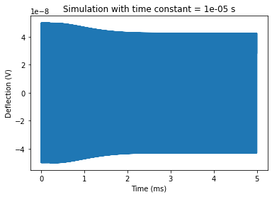
As you can see, the cantilever is going well, then at halfway there’s a change due to an exponential voltage pulse with time constant 10 ns. Let’s see what happens if we change the initial conditions.

Z, info = cant.simulate(Z0 = [0,0])
plt.plot(cant.t_Z * 1e3, Z)
plt.xlabel('Time (ms)')
plt.ylabel('Deflection (V)')
plt.title('Simulation with initial conditions 0 m, 0 m/s')

Text(0.5, 1.0, 'Simulation with initial conditions 0 m, 0 m/s')

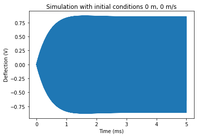
What happened?

Well, because we specified the cantilever to be at rest at time t=0 (Z0 = [0,0]), the cantilever had to oscillate for awhile before it settled at its steady-state condition. This initial part of the simulation is not all that useful, and it just wastes time, so we set the initial conditions.

Now, what if we change up some of the parameters? Let’s try a different time constant, maybe of 1e-3 s (1 ms).

cant.func_args = [1e-3]

In the cantilever, we will call a function that applies a single exponential decay to the voltage. That function requires a parameter, which we supply in the func_args list.

We can use this approach for** bi-exponential **and **stretched exponentials** as well.

Below, we will change the time constant to 1e-8 s, 1e-4 s, and 1e-2 s and see the result

# This is how you might change the time constant
cant.tau = 1e-3

fig, a = plt.subplots(nrows=3, ncols = 2, figsize=(12,14))

cant.tau = 1e-8
cant.func_args = [cant.tau]
Z, info = cant.simulate()
a[0][0].plot(cant.t_Z * 1e3, Z, 'b')
a[0][1].plot(cant.t_Z * 1e3, Z, 'b')
a[0][0].set_ylabel('Deflection (V), 10 ns')
a[0][0].set_title('Simulation with time constant = ' + str(cant.tau) + ' s')
a[0][1].set_title('Zooming in on the trigger time')
a[0][1].set_xlim(0.18, 0.5)
a[0][1].set_ylim(0.9, 1)

cant.tau = 1e-4
cant.func_args = [cant.tau]
Z, info = cant.simulate()
a[1][0].plot(cant.t_Z * 1e3, Z, 'b')
a[1][1].plot(cant.t_Z * 1e3, Z, 'b')
a[1][0].set_ylabel('Deflection (V), 100 us')
a[1][0].set_title('Simulation with time constant = ' + str(cant.tau) + ' s')
a[1][1].set_xlim(0.18, 0.5)
a[1][1].set_ylim(0.9, 1)

cant.tau = 1e-2
cant.func_args = [cant.tau]
Z, info = cant.simulate()
a[2][0].plot(cant.t_Z * 1e3, Z, 'b')
a[2][1].plot(cant.t_Z * 1e3, Z, 'b')
a[2][0].set_ylabel('Deflection (V), 10 ms')
a[2][0].set_title('Simulation with time constant = ' + str(cant.tau) + ' s')
a[2][1].set_xlim(0.18, 0.5)
a[2][1].set_ylim(0.9, 1)

a[2][0].set_xlabel('Time (ms)')
a[2][1].set_xlabel('Time (ms)')

# Add a line to mark the trigger at each point
trigger_line = np.linspace(-1.1, 1.1, 10)
a[0][0].plot(np.ones(len(trigger_line))*cant.trigger * 1e3, trigger_line, 'r-.')
a[1][0].plot(np.ones(len(trigger_line))*cant.trigger * 1e3, trigger_line, 'r-.')
a[2][0].plot(np.ones(len(trigger_line))*cant.trigger * 1e3, trigger_line, 'r-.')

[<matplotlib.lines.Line2D at 0x7fc33da932b0>]

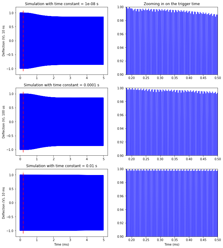
What happened?

Here, we are changing how quickly the resonance frequency changes. In the 10 ns and 100 us case, the cantilever looks similar. However, the key is what’s happening at the trigger time. For the 10 ns case, there’s a sharp change at the trigger (~1.6 ms). For the 100 us case, it’s a slow change. For the 10 ms case, there’s barely any change.

That means the interesting dynamics are in this region of the time window. The cantilevers in all three cases “relax” at about the same rate, because that is just dependent upon the cantilever Q factor for the most part, and it is unrelated to any transient effect.

Finally, let’s try changing the electrostatic force and the delta_freq (the amount of electrostatic force applied, i.e. the voltage, and the amount the resonance frequency shifts by). These values should normally not be changed independently as they’re related to one another and are acquired during a measurement. But, just for fun, let’s see what happens.

fig, a = plt.subplots(nrows=3, figsize=(6, 11))

cant.tau = 1e-6
cant.func_args = [cant.tau]
cant.es_force = 4e-9
cant.delta_freq = -170
cant.delta_w = 2* np.pi * cant.delta_freq # convert to radians
Z, info = cant.simulate()
a[0].plot(cant.t_Z * 1e3, Z, 'g')
a[0].set_ylabel('Deflection (V), Fe = 4 nN')
a[0].set_title('Changing Force, Fe = 4 nN, -170 Hz shift')

cant.es_force = 4e-7 # 100 X the force
cant.delta_freq = -170 # 600 Hz is a huge shift
cant.delta_w = 2* np.pi * cant.delta_freq # convert to radians
Z, info = cant.simulate()
a[1].plot(cant.t_Z * 1e3, Z, 'g')
a[1].set_ylabel('Deflection (V), Fe = 40 nN')
a[1].set_title('Changing Force, Fe = 40 nN, -170 Hz shift')

cant.es_force = 4e-9
cant.delta_freq = -600 # 600 Hz is a huge shift
cant.delta_w = 2* np.pi * cant.delta_freq # convert to radians
Z, info = cant.simulate()
a[2].plot(cant.t_Z * 1e3, Z, 'g')
a[2].set_ylabel('Deflection (V)')
a[2].set_xlabel('Time (ms)')
a[2].set_title('Changing Force, Fe = 40 nN, -600 Hz shift')

# Add a line to mark the trigger at each point
trigger_line = np.linspace(-1.1, 1.1, 10)
a[0].plot(np.ones(len(trigger_line))*cant.trigger * 1e3, trigger_line, 'r-.')
a[1].plot(np.ones(len(trigger_line))*cant.trigger * 1e3, trigger_line, 'r-.')
a[2].plot(np.ones(len(trigger_line))*cant.trigger * 1e3, trigger_line, 'r-.')

[<matplotlib.lines.Line2D at 0x7fc33d8257b8>]

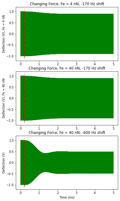
As you can see, the Electrostatic Force alone doesn’t do too much. The change in resonance frequency, though, changes a lot! This effect is because the change in resonance frequency changes the factors proportional to z and z’ in the DDHO equation.

## Changing the Excitation

We can supply a range of functions and parameters to the MechanicalDrive object to change the parameters of the simulation.

In the excitation.py file there are several different excitation functions listed. These are (currently) * single exponential * biexponential (sum) * stretched exponential

We can also supply an arbitrary excitation as long as it is scaled from 0 to 1. I’ll go through an example of each.

This is actually the default case. But, let’s go through it explicitly:

# Create a cantilever using single exponential change to resonance, 1 ms tau
params = [can_params, force_params, sim_params]
MechanicalDrive(*params, func = excitation.single_exp, func_args=[1e-3])

func is any callable function. What this does is apply a change such that omega_0 and Fe (resonance frequency, electrostatic force) are multiplied by this function once the trigger occurs.

cant = MechanicalDrive(can_params, force_params, sim_params, func=excitation.single_exp, func_args=[1e-3])

time_axis = np.arange(cant.trigger, cant.total_time, 1/cant.sampling_rate)
tau = 1e-3
exc_function = excitation.single_exp(time_axis - cant.trigger, tau)

fig, ax = plt.subplots(nrows=3, figsize=(8,16))

Z, _ = cant.simulate()
ax[0].plot(cant.t_Z, Z, 'b')
ax[0].plot(time_axis, exc_function, 'r--', linewidth=5)
ax[0].set_title('Single exponential change with tau = ' + str(tau) + ' s')
ax[0].set_xlabel('Time (s)')

# Change tau and resimulate
tau = 1e-2
cant.func_args = [tau]
exc_function = excitation.single_exp(time_axis - cant.trigger, tau)

Z, _ = cant.simulate()
ax[1].plot(cant.t_Z, Z, 'b')
ax[1].plot(time_axis, exc_function, 'g--', linewidth=5)
ax[1].set_title('Single exponential change with tau = ' + str(tau) + ' s')
ax[1].set_xlabel('Time (s)')

# Change tau and resimulate
tau = 1e-5
cant.func_args = [tau]
exc_function = excitation.single_exp(time_axis - cant.trigger, tau)

Z, _ = cant.simulate()
ax[2].plot(cant.t_Z, Z, 'b')
ax[2].plot(time_axis, exc_function, 'k--', linewidth=5)
ax[2].set_title('Single exponential change with tau = ' + str(tau) + ' s')
ax[2].set_xlabel('Time (s)')

# Add a line to mark the trigger at each point
trigger_line = np.linspace(-1.1, 1.1, 10)
ax[0].plot(np.ones(len(trigger_line))*cant.trigger, trigger_line, 'r-.')
ax[1].plot(np.ones(len(trigger_line))*cant.trigger, trigger_line, 'r-.')
ax[2].plot(np.ones(len(trigger_line))*cant.trigger, trigger_line, 'r-.')

[<matplotlib.lines.Line2D at 0x7fc33d5b04e0>]

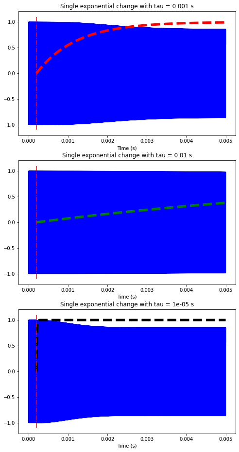
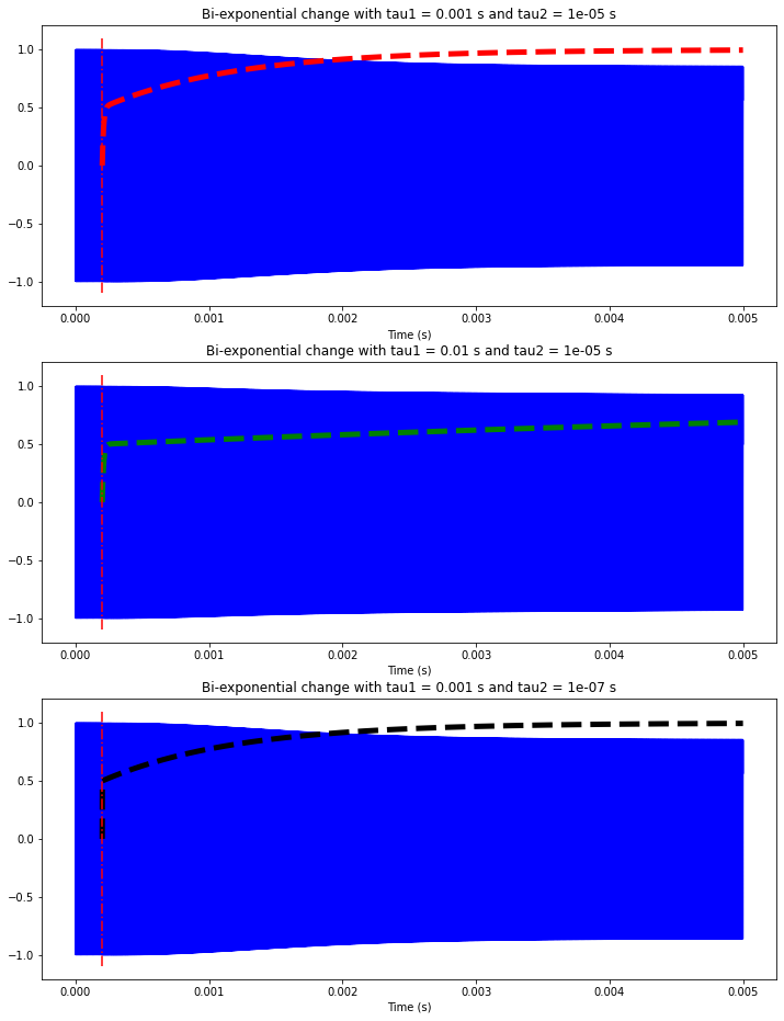
These functions are also included in the file excitation.py and can be easily added. They’re called “bi_exp” and “str_exp”

If you already have a cantilever, you need to change two things: 1. cant.func 2. cant.func_args

You can also change these when calling the function in the first place.

# Bi-exponential with tau1 = 1e-3 and tau2 = 1e-5
cant = MechanicalDrive(can_params, force_params, sim_params, func=excitation.bi_exp, func_args=[1e-3, 1e-5])

time_axis = np.arange(cant.trigger, cant.total_time, 1/cant.sampling_rate)
exc_function = excitation.bi_exp(time_axis - cant.trigger, *cant.func_args)

fig, ax = plt.subplots(nrows=3, figsize=(12,16))

Z, _ = cant.simulate()
ax[0].plot(cant.t_Z, Z, 'b')
ax[0].plot(time_axis, exc_function, 'r--', linewidth=5)
ax[0].set_title('Bi-exponential change with tau1 = ' + str(cant.func_args[0]) + ' s and tau2 = ' + str(cant.func_args[1]) + ' s')
ax[0].set_xlabel('Time (s)')

# Change tau1 to 1e-2
cant.func_args = [1e-2, 1e-5]
exc_function = excitation.bi_exp(time_axis - cant.trigger, *cant.func_args)

Z, _ = cant.simulate()
ax[1].plot(cant.t_Z, Z, 'b')
ax[1].plot(time_axis, exc_function, 'g--', linewidth=5)
ax[1].set_title('Bi-exponential change with tau1 = ' + str(cant.func_args[0]) + ' s and tau2 = ' + str(cant.func_args[1]) + ' s')
ax[1].set_xlabel('Time (s)')

# Change tau2 to 1e-7 and tau1 to 1e-3
cant.func_args = [1e-3, 1e-7]
exc_function = excitation.bi_exp(time_axis - cant.trigger, *cant.func_args)

Z, _ = cant.simulate()
ax[2].plot(cant.t_Z, Z, 'b')
ax[2].plot(time_axis, exc_function, 'k--', linewidth=5)
ax[2].set_title('Bi-exponential change with tau1 = ' + str(cant.func_args[0]) + ' s and tau2 = ' + str(cant.func_args[1]) + ' s')
ax[2].set_xlabel('Time (s)')

# Add a line to mark the trigger at each point
trigger_line = np.linspace(-1.1, 1.1, 10)
ax[0].plot(np.ones(len(trigger_line))*cant.trigger, trigger_line, 'r-.')
ax[1].plot(np.ones(len(trigger_line))*cant.trigger, trigger_line, 'r-.')
ax[2].plot(np.ones(len(trigger_line))*cant.trigger, trigger_line, 'r-.')

[<matplotlib.lines.Line2D at 0x7fc33d445b70>]

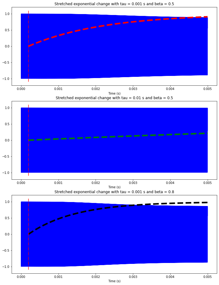
This can be modified in the same way, except that now:

cant.func_args = [tau, beta]

You can also change these when calling the function in the first place, like above.

# Stretched exponential with tau = 1e-3 and beta=0.5
cant = MechanicalDrive(can_params, force_params, sim_params, func=excitation.str_exp, func_args=[1e-3, 0.5])

time_axis = np.arange(cant.trigger, cant.total_time, 1/cant.sampling_rate)
exc_function = excitation.str_exp(time_axis - cant.trigger, *cant.func_args)

fig, ax = plt.subplots(nrows=3, figsize=(12,16))

Z, _ = cant.simulate()
ax[0].plot(cant.t_Z, Z, 'b')
ax[0].plot(time_axis, exc_function, 'r--', linewidth=5)
ax[0].set_title('Stretched exponential change with tau = ' + str(cant.func_args[0]) + ' s and beta = ' + str(cant.func_args[1]))
ax[0].set_xlabel('Time (s)')

# Change tau to 1e-5, keep beta the same
cant.func_args = [1e-2, 0.5]
exc_function = excitation.str_exp(time_axis - cant.trigger, *cant.func_args)

Z, _ = cant.simulate()
ax[1].plot(cant.t_Z, Z, 'b')
ax[1].plot(time_axis, exc_function, 'g--', linewidth=5)
ax[1].set_title('Stretched exponential change with tau = ' + str(cant.func_args[0]) + ' s and beta = ' + str(cant.func_args[1]))
ax[1].set_xlabel('Time (s)')

# Change tau back to 1e-3, make beta 0.85
cant.func_args = [1e-3, 0.8]
exc_function = excitation.str_exp(time_axis - cant.trigger, *cant.func_args)

Z, _ = cant.simulate()
ax[2].plot(cant.t_Z, Z, 'b')
ax[2].plot(time_axis, exc_function, 'k--', linewidth=5)
ax[2].set_title('Stretched exponential change with tau = ' + str(cant.func_args[0]) + ' s and beta = ' + str(cant.func_args[1]))
ax[2].set_xlabel('Time (s)')

# Add a line to mark the trigger at each point
trigger_line = np.linspace(-1.1, 1.1, 10)
ax[0].plot(np.ones(len(trigger_line))*cant.trigger, trigger_line, 'r-.')
ax[1].plot(np.ones(len(trigger_line))*cant.trigger, trigger_line, 'r-.')
ax[2].plot(np.ones(len(trigger_line))*cant.trigger, trigger_line, 'r-.')

[<matplotlib.lines.Line2D at 0x7fc33d35ff60>]

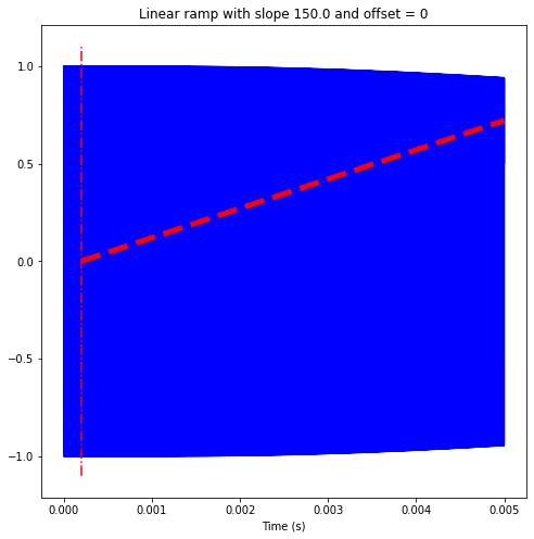
You can easily supply an arbitrary function, as long as you provide the relevant parameters.

def new_function(t, tau, tau2, tau3):
    return t * tau1 + t * tau2**2 - tau3

cant = MechanicalDrive(*params, func=new_function, func_args=[tau, tau2, tau3])

You can also directly change these after the cant object exists:

cant.func = new_functon
cant.func_args = [tau, tau2, tau3]

Note that the function *should scale from 0 to 1* to work.

Let’s try a quick example with a linear ramp.

def linear_ramp(t, slope, yoffset):

  return slope*t + yoffset

cant = MechanicalDrive(can_params, force_params, sim_params, func=linear_ramp, func_args=[1.5e2, 0])

time_axis = np.arange(cant.trigger, cant.total_time, 1/cant.sampling_rate)
exc_function = linear_ramp(time_axis - cant.trigger, *cant.func_args)

fig, ax = plt.subplots(figsize=(8, 8))

Z, _ = cant.simulate()
ax.plot(cant.t_Z, Z, 'b')
ax.plot(time_axis, exc_function, 'r--', linewidth=5)
ax.set_title('Linear ramp with slope ' + str(cant.func_args[0]) + ' and offset = ' + str(cant.func_args[1]))
ax.set_xlabel('Time (s)')

# Add a line to mark the trigger at each point
trigger_line = np.linspace(-1.1, 1.1, 10)
ax.plot(np.ones(len(trigger_line))*cant.trigger, trigger_line, 'r-.')

[<matplotlib.lines.Line2D at 0x7fc33c88b278>]

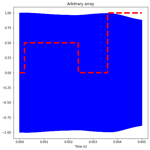
Lastly, you can also just directly supply the scaling yourself. This is passed differently, using parameter v_array

v_array must be the same sampling rate and length as the time axis you are simulating over.

This process requires a little thought. You could create a simple numpy array that’s the length you want if you know the parameters total_time and sampling_rate. If you multiply a time by a sampling_rate, you get an index of an array.

# Supply an arbitrary voltage array that effectively turns off the drive_frequency
print(sim_params)
arb_array = np.zeros(int(sim_params['sampling_rate']*sim_params['total_time']))
trigger_index = int(sim_params['trigger'] * sim_params['sampling_rate'])
half_index = int(0.5* (sim_params['total_time'] - sim_params['trigger']) * sim_params['sampling_rate'])
threefourths_index = int(0.75* (sim_params['total_time'] - sim_params['trigger']) * sim_params['sampling_rate'])
arb_array[trigger_index:half_index] = 0.5
arb_array[half_index:threefourths_index] = 0
arb_array[threefourths_index:] = 1

cant = MechanicalDrive(can_params, force_params, sim_params, v_array=arb_array)
time_axis = np.arange(0, cant.total_time, 1/cant.sampling_rate)
fig, ax = plt.subplots(figsize=(8, 8))

Z, _ = cant.simulate()
ax.plot(cant.t_Z, Z, 'b')
ax.plot(time_axis, arb_array, 'r--', linewidth=5)
ax.set_title('Arbitrary array')
ax.set_xlabel('Time (s)')

{'trigger': 0.0002, 'total_time': 0.005, 'sampling_rate': 10000000.0}

Text(0.5, 0, 'Time (s)')